Using VLOOKUP can be a little scary at first, but it’s an extremely useful formula that should be in the arsenal of every data manager!
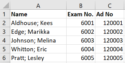
If you have data in two lists in Excel, like these:
 |
 |
And they have a consistent column of data between them (in this case exam number), you can use this consistent column to merge the two lists. In this example, I want to add the admission number in the second list to the first.
Firstly, I’ll add an empty column to the first spreadsheet:

I then need to add the following formula to cell C2 "=VLOOKUP(A2,Lookup!B1:C6,2,FALSE)“:
You'll see shortly that the final formula is a little different to this, I'll explain why in a moment. The important thing is that I didn't actually type the majority of that formula, this is how I created it:
-
Type =VLOOKUP(
-
Excel is now looking for a cell reference for the value you want to look up in the second list (exam number), which you can supply by clicking on the relevant cell, so I clicked on cell A2. The formula is now =VLOOKUP(A2

-
I now type a comma to move to the next part of the formula.
-
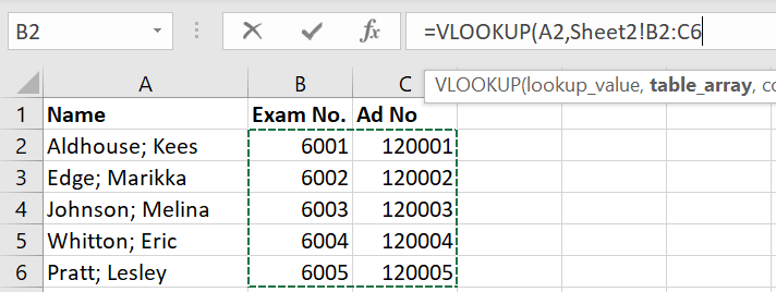
Excel now wants the array you want to use in the formula, again you can give it this by selecting the cells rather than typing the values. My list is in sheet 2 of the same Excel workbook (although you can also click onto a completely separate Excel workbook here), so I clicked on the tab then dragged my mouse from cell B2 down to cell C6. The formula is now =VLOOKUP(A2,Sheet2!B2:C6

If you select cells in a different workbook entirely, rather than saying Sheet2! the name of the workbook will be displayed in quotation marks before the exclamation point. - Without clicking back to the initial tab, I now typed another comma.
- The next part of the formula asks for the column reference for the value you want to return from the range selected. I've picked B2 to C6 and there are two columns selected; the admission number is in the second column, so the value I entered here is 2, followed by another comma - =VLOOKUP(A2,Sheet2!B1:C6,2,
- The final 'False' part of the formula tells Excel to look for an exact match, I always use False here.
- Follow this with a bracket and click the tick icon to the left of the formula at the top of the screen in Excel. You'll now have the final formula =VLOOKUP(A2,Sheet2!B1:C6,2,FALSE)

There's one more thing to do before copying the formula down the rest of column C, you have to make the array an absolute reference otherwise Excel will automatically start referencing blank cells when you use auto-complete to copy the formula. To do this highlight the array reference in the formula (shown in bold):
=VLOOKUP(A2,Sheet2!B2:C6,2,FALSE)
Now press F4 (or possibly fn+F4 depending on your keyboard layout) once, you should see this:
=VLOOKUP(A2,Sheet2!$B$2:$C$6,2,FALSE)

These values are now absolutes and will stay the same when you copy the formula down the sheet. Make sure you click the tick again to confirm the formula, then hover over the small square in the bottom right hand corner of the cell containing the formula, and either double click or drag the formula down the page:

And that’s it, the two lists of data have been merged! Of course, you can use this for much more than just adding ID numbers for your students. For example, you could also use it to merge two completely separate lists of grades together, even if they contain different numbers of students. It’s always much quicker and safer than attempting these merges by eye!
Thanks for reading!
